
Inventory Control Models: EOQ Formulations & Selective Control Frameworks
1. The Economics of Inventory Management: Functions, Costs & Trade-Offs
Inventory represents any idle resource held for future use to facilitate operational flow or satisfy customer demand. In manufacturing and retail supply chains, inventory typically accounts for 20% to 40% of total enterprise assets, making its scientific management critical to liquidity and return on capital employed (ROCE).
The Three Conflicting Inventory Cost Categories:
- 1. Inventory Holding (Carrying) Costs (\(H\)): The expenses associated with storing unsold inventory over time, including: (a) Opportunity cost of capital (interest on funds tied up in stock — typically 12–18%), (b) Physical warehousing rent, utilities, and security, (c) Insurance premiums and inventory taxes, and (d) Deterioration, spoilage, shrinkage, breakage, and technological obsolescence. Total carrying cost typically ranges from 20% to 30% of the item’s unit value annually.
- 2. Ordering / Setup Costs (\(S\)): Fixed expenses incurred each time an order is placed or a factory machine is retooled, including: purchasing department clerical salaries, supplier billing processing, freight shipping documentation, quality receiving inspection, and shop-floor machine tooling teardown and reset.
- 3. Stockout (Shortage) Costs: Economic losses incurred when inventory is exhausted during demand, including: lost contribution margin on lost sales, emergency freight expediting penalties, customer goodwill destruction, and idle worker wages during factory line shutdowns.
2. The Classical Economic Order Quantity (EOQ) Model & Quantity Discounts
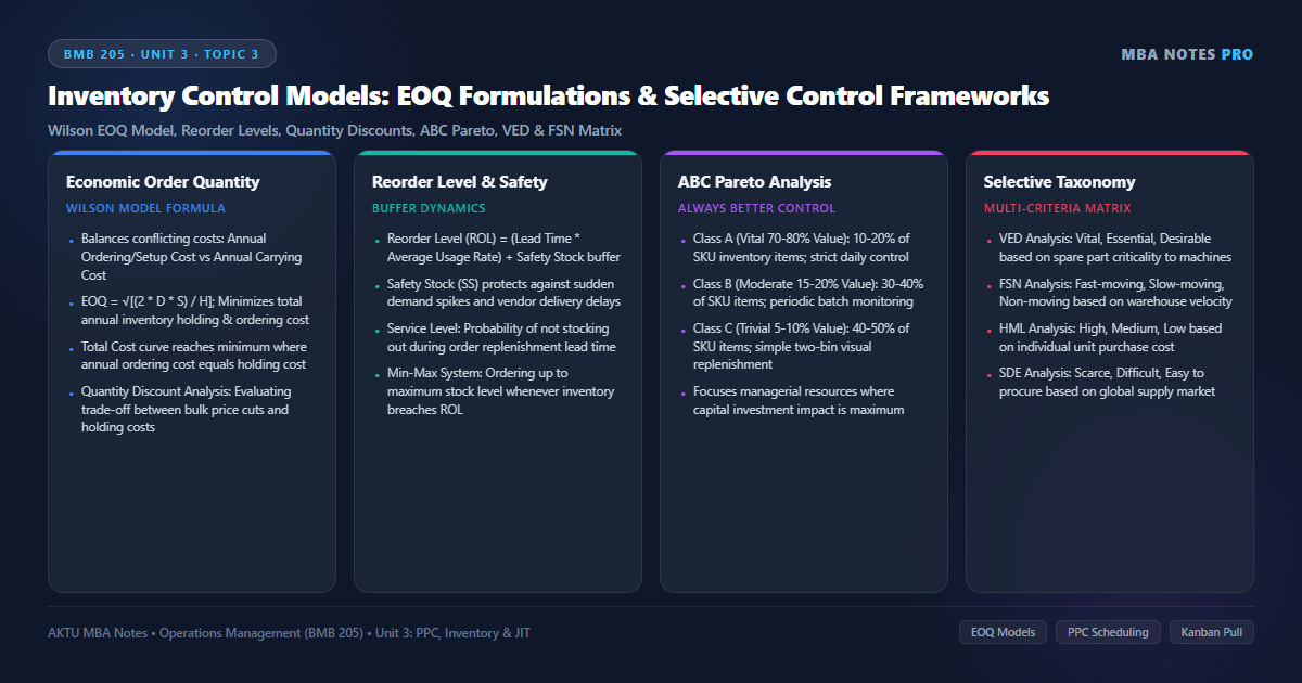
Developed by Ford W. Harris (1913) and popularized by R.H. Wilson, the Economic Order Quantity (EOQ) model determines the optimal order size that minimizes the total annual cost of ordering and holding inventory.
Where \(D\) = Annual demand (units); \(Q\) = Order quantity; \(S\) = Ordering/setup cost per order; \(H\) = Carrying cost per unit per year (or \(I \times C\), where \(I\) is carrying rate % and \(C\) is unit purchase price); \(d\) = Daily usage rate; \(L\) = Supplier lead time (days); and \(SS\) = Safety stock buffer.
Problem: Sunrise Pumps Ltd. requires 10,000 units of a mechanical seal annually (\(D = 10,000\)). The purchase cost per seal is ₹100 (\(C = 100\)). Ordering cost is ₹200 per order (\(S = 200\)), and inventory carrying cost is 20% of unit price per year (\(H = 0.20 \times 100 = ₹20\)). The supplier offers a 3% discount on the unit price if the order quantity is 2,500 units or more.
Calculate: (a) The standard EOQ, (b) Total annual inventory cost at EOQ, and (c) Evaluate whether Sunrise Pumps should accept the supplier’s quantity discount offer.
\(EOQ = \sqrt{\frac{2 \times D \times S}{H}} = \sqrt{\frac{2 \times 10,000 \times 200}{20}} = \sqrt{\frac{4,000,000}{20}} = \sqrt{200,000} = \mathbf{447.21 \approx 447 \text{ units}}\).
Step 2: Total Annual Cost at Standard EOQ (\(Q = 447\), \(C = ₹100\)):
• Material Purchase Cost: \(10,000 \times ₹100 = ₹10,00,000\)
• Annual Ordering Cost: \(\left(\frac{10,000}{447}\right) \times 200 = 22.37 \times 200 = ₹4,474\)
• Annual Holding Cost: \(\left(\frac{447}{2}\right) \times 20 = 223.5 \times 20 = ₹4,470\)
\(\text{Total Cost at EOQ} = ₹10,00,000 + ₹4,474 + ₹4,470 = \mathbf{₹10,08,944}\).
Step 3: Total Annual Cost with Quantity Discount (\(Q = 2,500\), Discounted Price \(C_{new} = ₹97\)):
• Discounted Unit Price: \(₹100 – (3\% \text{ of } ₹100) = ₹97\).
• New Unit Holding Cost (\(H_{new}\)): \(20\% \times ₹97 = ₹19.40\).
• Discounted Material Purchase Cost: \(10,000 \times ₹97 = ₹9,70,000\) (Savings of ₹30,000!)
• New Annual Ordering Cost: \(\left(\frac{10,000}{2,500}\right) \times 200 = 4 \times 200 = ₹800\)
• New Annual Holding Cost: \(\left(\frac{2,500}{2}\right) \times 19.40 = 1,250 \times 19.40 = ₹24,250\)
\(\text{Total Cost with Discount} = ₹9,70,000 + ₹800 + ₹24,250 = \mathbf{₹9,95,050}\).
Step 4: Strategic Managerial Decision:
\(\text{Net Annual Savings} = ₹10,08,944 – ₹9,95,050 = \mathbf{₹13,894}\).
Conclusion: Accept the supplier’s quantity discount! Even though annual carrying costs rise from ₹4,470 to ₹24,250, the massive ₹30,000 savings in direct material purchase cost yields a net enterprise profit increase of ₹13,894 per year.
3. Selective Inventory Control Frameworks: ABC, VED & FSN Analysis
Because an industrial manufacturing plant or hospital warehouse may store over 50,000 distinct SKU items, treating every item with identical managerial scrutiny is physically impossible. Selective Inventory Control classifies inventory items based on specific criteria to focus executive attention where working capital impact is greatest:
| Technique | Classification Criterion | Categorization Breakdown | Managerial Inventory Control Policy |
|---|---|---|---|
| ABC Analysis (Pareto Principle) | Annual Consumption Value (Quantity Consumed × Unit Price). | • Class A: 10–20% of items, accounting for 70–80% of total annual value. • Class B: 30–40% of items, accounting for 15–20% of value. • Class C: 40–50% of items, accounting for only 5–10% of value. | • Class A: Strict daily control, perpetual inventory tracking, minimal safety stock, JIT delivery. • Class B: Monthly batch review, moderate safety stock. • Class C: Simple two-bin visual control, bulk ordering, large safety stock. |
| VED Analysis | Criticality of spare parts to production machine operation. | • V — Vital: Absence completely shuts down entire production plant. • E — Essential: Absence causes severe operational degradation but not full stoppage. • D — Desirable: Absence causes minor inconvenience without affecting production. | • Vital: Maintain high safety stock regardless of unit cost; zero stockouts tolerated. • Essential: Moderate buffer stocks. • Desirable: Low stock; ordered as needed. |
| FSN Analysis | Turnover velocity and consumption frequency from warehouse. | • F — Fast-Moving: Issued frequently in high quantities. • S — Slow-Moving: Issued infrequently in small quantities. • N — Non-Moving: Zero issues for over 12–24 months (dead stock). | • Fast: Placed near warehouse loading docks for rapid picking. • Slow: Placed in upper racking. • Non-Moving: Liquidated, auctioned, or written off to liberate trapped capital. |
4. Specialized Inventory Taxonomies: HML, SDE, GOLF & The ABC-VED Matrix
Beyond the primary triad (ABC, VED, FSN), industrial procurement departments deploy specialized selective classification matrices:
A. Specialized Selective Classification Techniques:
- HML Analysis (High, Medium, Low Unit Cost): Classifies items strictly by unit purchase price (e.g., High > ₹1,000, Medium ₹200–₹1,000, Low < ₹200). Determines purchasing authorization limits (VP approval required for High-cost items).
- SDE Analysis (Scarce, Difficult, Easy Procurement): Classifies items based on market availability:
- Scarce (S): Imported items, canalized materials, or raw materials with sovereign supply quotas. Mandates maintaining 6–12 months of strategic stock.
- Difficult (D): Customized engineered components requiring long fabrication lead times.
- Easy (E): Off-the-shelf standard hardware (nuts, bolts, lubricants) available locally within 24 hours.
- GOLF Analysis (Government, Open Market, Local, Foreign): Classifies items by supply channel origin to assess procurement payment lead times and customs tariffs.
- SOS Analysis (Seasonal vs Off-Seasonal): Classifies agro-commodities based on harvesting seasons to execute bulk procurement during price troughs.
The Power of Cross-Classification: The ABC-VED Matrix:
By combining ABC Analysis (Financial Value) with VED Analysis (Operational Criticality) into a 3×3 matrix (AV, AE, AD, BV, BE, BD, CV, CE, CD), operations managers achieve ultimate inventory precision. An inexpensive ₹5 gasket that is Vital (CV) receives far tighter monitoring and safety stock than an expensive ₹50,000 aesthetic logo plate that is Desirable (AD)!
Corporate Case Vignette: Asian Paints’ Automated Inventory SCM & Point-of-Sale Tinting Decentralization
Asian Paints, India’s undisputed decorative coatings market leader with over 55% market share, transformed inventory control through one of the most celebrated operational innovations in Indian business history:
- The Inventory Proliferation Crisis: In the traditional paint industry, offering customers 2,000 distinct color shades in 4 different can sizes (1L, 4L, 10L, 20L) meant stocking over 8,000 distinct SKUs per retail dealership. Dealers suffered massive dead-stock write-offs in unpopular colors while stocking out of popular shades.
- The ‘Colour Idea’ Point-of-Sale Tinting Machine (Postponement): Asian Paints decentralized the final manufacturing stage to retail counters. Dealers stock only 4 standardized white base cans and computerized tinting colorants. When a homeowner selects a specific shade, the automated tinting machine dispenses the exact color formulation in 90 seconds.
- Enterprise AI Demand Sensing & Automated ROL: Asian Paints connects its 70,000+ retail tinting machines directly to central manufacturing plants. Every can dispensed automatically triggers a replenishment signal in the central ERP, generating dynamic EOQ deliveries 3 to 4 times a week.
- Measurable Impact: Finished goods inventory turns reached an extraordinary 3.5 days of finished inventory at regional distribution centers, achieving a 99.7% order fill rate while eliminating millions in obsolete inventory carrying costs.
Managerial Takeaway: Postponing product customization to the point of sale slashes SKU inventory holding costs by orders of magnitude while delivering infinite variety to consumers.
AKTU University Examination Questions: Inventory Control Techniques (EOQ & Selective Models)
Section A (2 Marks Conceptual Questions):
Q1: State the formula for Economic Order Quantity (EOQ) and define each term. (2 Marks)
Q2: Distinguish between ABC Analysis and VED Analysis. (2 Marks)
Section B / C (10 Marks Detailed Analytical Question):
Q: Explain the concept, assumptions, and cost trade-offs of the Classical EOQ model with a neat total cost graph. Detail the selective inventory control techniques: ABC, VED, FSN, and SDE. An enterprise has annual demand of 8,000 units, ordering cost of ₹180/order, and carrying cost of ₹4/unit/year. Calculate: (a) EOQ, (b) Number of orders per year, and (c) Total annual inventory holding and ordering cost. (10 Marks)
1. Inventory Costs & EOQ Concept: Explain trade-off between Annual Ordering Costs and Annual Holding Costs; draw the U-shaped Total Cost curve showing minimum at point where Ordering Cost = Holding Cost.
2. Selective Inventory Control Frameworks: Detail ABC Analysis (Pareto 70-20-10 value rule), VED Analysis (criticality of spares), FSN Analysis (warehouse movement speed), and SDE Analysis (procurement difficulty).
3. The ABC-VED 3×3 Matrix: Explain how cross-classifying value and criticality optimizes spare parts management.
4. Complete Step-by-Step Numerical Solution:
• \(EOQ = \sqrt{\frac{2 \times 8,000 \times 180}{4}} = \sqrt{\frac{2,880,000}{4}} = \sqrt{720,000} = \mathbf{848.53 \approx 849 \text{ units}}\).
• \(N = \frac{D}{EOQ} = \frac{8,000}{849} = \mathbf{9.42 \approx 10 \text{ orders/year}}\).
• \(\text{Annual Ordering Cost} = \left(\frac{8,000}{849}\right) \times 180 = 9.423 \times 180 = ₹1,696.14\).
• \(\text{Annual Holding Cost} = \left(\frac{849}{2}\right) \times 4 = 424.5 \times 4 = ₹1,698.00\).
• \(\text{Total Inventory Cost} = ₹1,696.14 + ₹1,698.00 = \mathbf{₹3,394.14}\).
5. Corporate Case Reference: Cite Asian Paints’ point-of-sale tinting machine postponement and automated replenishment.
Discussion & Questions
0 CommentsAcademic insights, questions, and conceptual clarifications from students & faculty.
No questions or comments yet
Have a doubt about this topic, an exam tip, or a conceptual perspective? Start the discussion below!
Leave a Comment / Ask a Question
Your email address will not be published. Required fields are marked *