
Quality Circles (QC), 7 Traditional QC Tools & 7 New Quality Management Tools
Frontline Problem Solving, Ishikawa’s 7 Statistical QC Tools & Advanced Management Planning Matrices
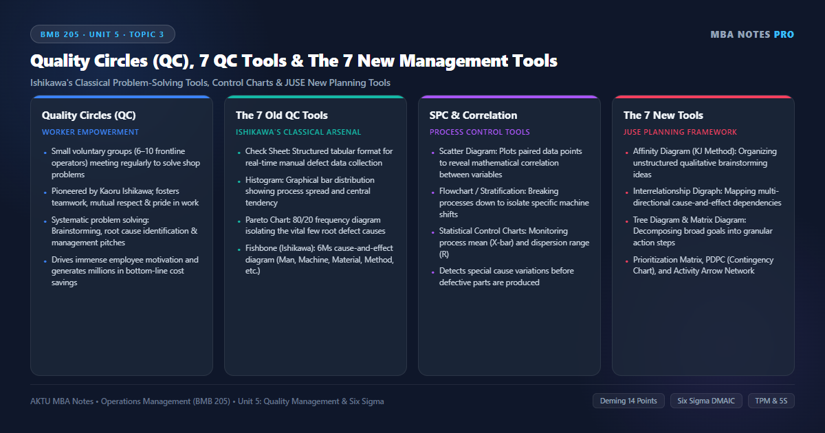
1. Quality Circles (QC): Concept, Structural Architecture & Working Dynamics
Quality Circles (QC) were pioneered in Japan in 1962 by Dr. Kaoru Ishikawa and the Union of Japanese Scientists and Engineers (JUSE). A Quality Circle is defined as a small, voluntary group of frontline employees from the same work area who meet periodically—typically one hour per week on company time—to identify, analyze, and solve work-related operational challenges.
Unlike ad-hoc task forces appointed by senior executives to solve specific crises, Quality Circles represent a permanent, bottom-up organizational vehicle for continuous improvement, employee empowerment, and human potential development.
Primary Objectives of Quality Circles
- Improve Operational Quality & Productivity: Systematically eliminate scrap, machine downtime, ergonomic bottlenecks, and procedural errors.
- Foster Frontline Problem-Solving Skills: Train shop-floor workers in statistical literacy, scientific causality, and presentation skills.
- Enhance Employee Morale & Teamwork: Transform routine, repetitive factory work into meaningful intellectual participation and collective pride.
- Bridge Industrial Relations: Create mutual trust and open communication between frontline operators and plant management.
- Cultivate Future Supervisors: Serve as an internal leadership incubator where circle leaders demonstrate initiative and team leadership.
The Organizational Structure of Quality Circles
- Steering Committee: Chaired by the Chief Executive or Plant Head, this body formulates quality circle policies, allocates operational budgets, and reviews program health.
- Facilitator: A senior manager or industrial engineer who coordinates multiple circles across departments, organizes training workshops, and liaises with executive leadership.
- Circle Leader: Usually chosen democratically by the circle members (often the line supervisor or a senior operator) to steer weekly agendas, maintain meeting discipline, and assign project tasks.
- Circle Members: 6 to 10 voluntary frontline operators who participate actively in brainstorming, data gathering, root cause diagnosis, and countermeasure execution.
- Non-Members: Adjacent shop-floor workers who cooperate with circle members during data collection and pilot testing of new procedures.
Comparative Matrix: The 7 Traditional QC Tools vs. The 7 New Quality Management Tools
| Operational Dimension | The 7 Traditional QC Tools (Old Tools) | The 7 New Management Tools (New Tools) |
|---|---|---|
| Origin & Pioneer | Pioneered in 1960s by Dr. Kaoru Ishikawa & JUSE | Developed in 1970s by JUSE Committee on Quality Tools |
| Primary Data Type | Quantitative, numerical, empirical measurement data | Qualitative, conceptual, verbal, and linguistic data |
| Target Organizational Tier | Shop-floor operators, line supervisors, maintenance crews | Middle managers, systems engineers, R&D planners |
| Operational Focus | Defect detection, variance analysis, process stabilization | Strategic planning, design conception, risk forecasting |
| Problem Complexity | Structured, operational, repetitive technical bottlenecks | Unstructured, strategic, cross-functional organizational dilemmas |
| Representative Tools | Check Sheet, Histogram, Pareto Chart, Fishbone, Control Chart | Affinity (KJ), Relations, Tree, Matrix, PDPC, Arrow Diagram |
| Core Analytical Goal | Discover root causes and control process variation | Organize chaotic ideas, prioritize actions, map dependencies |
2. The 7 Traditional Quality Control (QC) Tools: Step-by-Step Analysis
Dr. Kaoru Ishikawa asserted that over 95% of all shop-floor operational problems can be resolved using seven fundamental graphical and statistical tools. These are universally known as the 7 QC Tools.
1. Check Sheet (Tally Sheet)
A simple, structured data collection form designed to record observed defect counts or event occurrences in real-time. By providing predefined categories and check marks, it standardizes shop-floor data collection and prevents recording bias.
2. Histogram
A frequency distribution bar chart that visualizes the spread, central tendency, and shape of a continuous dataset (e.g., component diameters, filling weights). It instantly reveals whether a process is normally distributed, skewed, bimodal, or running uncomfortably close to specification limits.
3. Pareto Diagram (The 80/20 Rule)
Named after Vilfredo Pareto and adapted by Joseph Juran, the Pareto chart combines a descending bar chart of defect categories with a cumulative percentage line. It separates the ‘vital few’ causes (20% of defect types that cause 80% of total losses) from the ‘useful many’, ensuring engineers prioritize the most damaging bottlenecks.
4. Cause-and-Effect Diagram (Fishbone / Ishikawa Diagram)
A graphical brainstorming tool that organizes potential causes of a specific quality problem (the fish head) along main diagonal structural bones. In manufacturing, these causes are systematically categorized under the 6Ms:
- Man (People): Operator training, fatigue, skill level, absenteeism, adherence to SOPs.
- Machine: Equipment age, spindle play, calibration drift, tooling wear, lubrication.
- Material: Chemical composition, supplier grade, moisture content, tensile strength.
- Method: Standard work procedures, cutting speeds, sequence of operations, cycle timing.
- Measurement: Gauge accuracy, measurement bias, parallax error, calibration frequency.
- Milieu (Mother Nature / Environment): Ambient shop-floor temperature, humidity, lighting, vibration.
5. Scatter Diagram
A mathematical plot displaying paired data points $(X, Y)$ on a Cartesian grid to analyze the correlation between an independent process variable (e.g., sintering furnace temperature) and a dependent quality characteristic (e.g., ceramic hardness). It identifies positive, negative, or zero relationships.
6. Stratification (or Flowchart)
A data-sorting technique that separates mixed operational data into homogeneous subgroups based on specific factors (e.g., shift timing, machine line, operator experience, vendor lot). Stratification reveals hidden patterns that are obscured when all data is lumped together.
7. Statistical Process Control (SPC) Charts
Pioneered by Walter Shewhart, control charts plot sequential sample statistics over time against a Central Line (CL), Upper Control Limit (UCL), and Lower Control Limit (LCL). They distinguish between natural common cause variation (inherent in the process) and assignable special cause variation (requiring immediate intervention).
3. The 7 New Quality Management & Planning Tools
As quality management expanded from shop-floor manufacturing into product design, strategic planning, and service delivery, JUSE introduced the 7 New Management Tools in 1976 to help managers analyze complex, unstructured qualitative information.
1. Affinity Diagram (The KJ Method)
Developed by anthropologist Jiro Kawakita, this tool groups large volumes of chaotic, unstructured verbal ideas, opinions, and customer feedback into natural categories based on instinctive affinity or thematic similarity.
2. Relations Diagram (Interrelationship Diagraph)
Maps complex, multidirectional cause-and-effect relationships among diverse problem factors using arrows. Factors with the most outgoing arrows are identified as fundamental root drivers; factors with the most incoming arrows are primary bottlenecks.
3. Tree Diagram
A hierarchical branching diagram that breaks down broad strategic objectives into increasingly granular sub-goals, tasks, and implementation steps (e.g., mapping corporate customer delight goals into specific workstation procedures).
4. Matrix Diagram
A multi-dimensional grid (L-shaped, T-shaped, or X-shaped) that evaluates the strength of relationships between two or more sets of factors (e.g., correlating customer requirements against engineering technical specifications in Quality Function Deployment / House of Quality).
5. Matrix Data Analysis (Prioritization Matrix)
The only numerical tool among the new seven; it applies principal component analysis and weighted scoring to rank competing options across multiple objective criteria.
6. Process Decision Program Chart (PDPC)
A proactive risk assessment flowchart that systematically identifies potential pitfalls, failures, and disruptions during the execution of a complex plan, mapping contingency countermeasures beforehand.
7. Arrow Diagram (Activity Network Diagram)
Essentially the Critical Path Method (CPM) / PERT network; it sequences project activities, establishes task interdependencies, and identifies the critical path to ensure optimal project completion timing.
Statistical Process Control: X-Bar & R Control Limits & Solved Numerical Problem
Variables & Notation:
- \bar{\bar{X}}: Grand mean of all subgroup sample averages
- \bar{R}: Average range across all recorded sample subgroups
- A_2: Statistical factor for X-bar chart control limits based on subgroup size n
- D_3, D_4: Statistical factors for Range (R) chart control limits based on subgroup size n
- \text{UCL}, \text{LCL}: Upper Control Limit and Lower Control Limit (±3 Sigma boundaries)
Step-by-Step Solved Problem Illustration:
- A precision gear manufacturer monitors shaft diameters. Over 20 consecutive production subgroups of size n = 5 parts each, the quality inspector records: Sum of sample means (Σ X-bar) = 700.00 mm, and Sum of sample ranges (Σ R) = 42.00 mm. For subgroup size n = 5, statistical table factors are: A_2 = 0.577, D_3 = 0, D_4 = 2.115.
- Step 1: Calculate the Grand Mean (X-double-bar) = (Σ X-bar) / k = 700.00 / 20 = 35.00 mm.
- Step 2: Calculate the Average Range (R-bar) = (Σ R) / k = 42.00 / 20 = 2.10 mm.
- Step 3: Calculate Range (R) Chart Control Limits: CL_R = 2.10 mm; UCL_R = D_4 × R-bar = 2.115 × 2.10 = 4.4415 mm; LCL_R = D_3 × R-bar = 0 × 2.10 = 0.00 mm.
- Step 4: Calculate X-Bar Chart Control Limits: CL_X = 35.00 mm; UCL_X = X-double-bar + (A_2 × R-bar) = 35.00 + (0.577 × 2.10) = 35.00 + 1.2117 = 36.2117 mm; LCL_X = X-double-bar – (A_2 × R-bar) = 35.00 – 1.2117 = 33.7883 mm.
- Operational Conclusion: The process is in statistical control if all 20 sample means fall between 33.79 mm and 36.21 mm, and all sample ranges remain below 4.44 mm.
4. Statistical Process Control: Out-of-Control Patterns & Rules of Interpretation
Simply calculating control limits is insufficient; operations managers must be able to interpret chart behavior. A process is considered out of statistical control (indicating an assignable cause) if any of the following Western Electric Rules occur:
- Single Point Outside Limits: Any single sample point falls above the Upper Control Limit (UCL) or below the Lower Control Limit (LCL).
- Rule of Seven (Run of Points): Seven or more consecutive sample points fall on one side of the central line, indicating a process shift.
- Trending Sequence: Six or more consecutive points steadily increasing or steadily decreasing, indicating progressive tool wear or temperature drift.
- Hugging the Center Line: Fifteen consecutive points falling within ±1 Sigma of the center line, indicating over-stratification or fabricated data.
- Cycling or Periodicity: Regular oscillating waves, indicating operator shift rotation or ambient cooling-cycle influences.
Quality Circles Architecture
Voluntary shop-floor teams supported by Facilitators and Steering Committees to solve local problems.
The 7 Old QC Tools
Empirical tools: Check Sheet, Histogram, Pareto (80/20), Fishbone (6M), Scatter, Flowchart, Control Charts.
The 7 New Management Tools
Conceptual matrices: Affinity (KJ), Relations, Tree, Matrix, Prioritization, PDPC, and Arrow Networks.
Statistical Process Control
3-Sigma control limits (X-bar and R charts) monitoring common vs assignable process variation.
6. Corporate Case Vignette: Corporate Case Vignette: Bharat Electronics Limited (BEL) Quality Circles
Background: Bharat Electronics Limited (BEL), a premier Indian Navratna defense public sector enterprise, manufactures state-of-the-art radar, sonar, and electronic warfare systems for the Indian Armed Forces. In defense manufacturing, component failure can compromise national security; thus, component reliability tolerances are unforgiving.
The QC Intervention: BEL instituted a nationwide Quality Circle movement across its Bangalore, Ghaziabad, and Kotdwara complexes. Operating under names like ‘Radar Sparx’ and ‘Precision Pioneers’, circles executed structured problem-solving projects:
- Fishbone Diagnosis on SMT Lines: Circle members investigated solder bridging defects on printed circuit boards (PCBs). Using an Ishikawa diagram, they isolated the root cause to stencil aperture thickness and solder paste viscosity rather than operator handling.
- Pareto Analysis on Mechanical Housings: Analyzed 14 defect categories on radar radome composite machining. The Pareto chart revealed that two defects—delamination and fastener hole burrs—accounted for 84% of all rework costs.
- Poka-Yoke Fixture Innovation: Circle members designed an inexpensive magnetic jig that mechanically prevented reversed diode insertion during cable harness assembly.
Strategic Results: BEL’s Quality Circles have represented India at international QC conventions (ICQCC) across Japan, Korea, and Singapore, repeatedly winning Gold awards. Solder defect rates on critical radar assemblies plummeted from 1,200 PPM to under 45 PPM, saving millions in rework while ensuring zero-defect mission reliability for frontline defense systems.
7. AKTU Previous Years Questions & Model Solutions
The following questions reflect the standard question patterns, marks distribution, and evaluation criteria of Dr. A.P.J. Abdul Kalam Technical University (AKTU) MBA Semester Examinations.
A Quality Circle is a voluntary group of 6 to 10 frontline workers from the same work area who meet periodically to identify, analyze, and solve work-related quality and productivity problems. Dr. Kaoru Ishikawa pioneered the Quality Circle concept in Japan in 1962.
The 6Ms used in an Ishikawa diagram are: Man (People), Machine (Equipment), Material (Raw inputs), Method (Procedures/Process), Measurement (Inspection/Gauges), and Milieu or Mother Nature (Workplace Environment).
The 7 Old QC Tools are primarily quantitative, numerical, and data-driven, used by shop-floor operators to analyze and stabilize processes. The 7 New Management Tools are qualitative, verbal, and conceptual, used by managers and planners to organize complex ideas and strategize implementation.
Model Answer Structure:
1. Introduction: Origin of the 7 QC Tools by Kaoru Ishikawa; purpose of enabling non-mathematicians to analyze data.
2. Comprehensive Breakdown of all 7 Tools:
– Check Sheet: Concept, purpose, tally illustration.
– Histogram: Frequency distribution, bell curve comparison, spec limit evaluation.
– Pareto Diagram: 80/20 rule, vital few vs useful many, cumulative percentage curve.
– Cause-and-Effect Diagram: Fishbone structure, problem statement at head, detailed 6M categorization.
– Scatter Diagram: X-Y correlation, positive/negative/zero patterns.
– Stratification / Flowchart: Subgroup separation by shift/vendor, process step mapping.
– Control Charts: UCL, LCL, Center line, X-bar and R chart applications.
3. Empowerment Mechanism: Explain how these visual tools eliminate guesswork, enable fact-based problem solving at the operator level, and support Quality Circles.
4. Corporate Example: Cite BEL or Maruti Suzuki Quality Circle achievements.
5. Conclusion: Reiterate that mastery of these 7 tools forms the bedrock of Statistical Process Control and World-Class Manufacturing.
Discussion & Questions
0 CommentsAcademic insights, questions, and conceptual clarifications from students & faculty.
No questions or comments yet
Have a doubt about this topic, an exam tip, or a conceptual perspective? Start the discussion below!
Leave a Comment / Ask a Question
Your email address will not be published. Required fields are marked *