
Analysis of Variance (ANOVA): One-Way & Two-Way Classifications
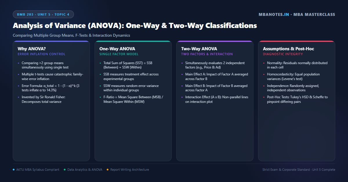
1. The Conceptual Rationale: Why t-Tests Fail for Multiple Groups
When business researchers compare two groups (e.g., sales performance of Male vs Female sales reps), a two-sample t-test is the appropriate statistical tool. However, corporate managers routinely evaluate three, four, or more groups (e.g., comparing productivity across Delhi, Mumbai, Bangalore, and Chennai offices). Conducting pairwise t-tests across multiple groups leads to severe statistical contamination known as Family-Wise Type I Error Inflation.
To compare k = 4 groups, the number of pairwise comparisons is C = k(k − 1)/2 = 4(3)/2 = 6 t-tests.
The overall probability of committing at least one Type I error (αFW) across 6 independent tests at α = 0.05 is:
αFW = 1 − (1 − α)C = 1 − (1 − 0.05)6 = 1 − (0.95)6 = 1 − 0.735 = 0.265 (26.5%)!
Instead of a 5% false alarm risk, the researcher now has a catastrophic 26.5% chance of falsely reporting a significant finding!
The Fisherian Solution: Analysis of Variance (ANOVA):
- Single Omnibus Test: Invented by Sir Ronald A. Fisher, ANOVA tests for differences among all group means simultaneously in a single statistical test, preserving the overall Type I error rate strictly at α = 0.05.
- Comparing Variances to Compare Means: Although the research objective is to test whether group means are equal, the mathematical vehicle used is the comparison of variance estimates (hence the name 'Analysis of Variance').
- Null Hypothesis of ANOVA: Always states that all population means are equal: H₀: μ₁ = μ₂ = μ₃ = ... = μk.
- Alternative Hypothesis of ANOVA: States that at least one group mean is different from the others (it does not require all means to be different).
- The F-Distribution: Named in honor of Sir Ronald Fisher, the F-distribution is a positively skewed continuous probability distribution representing the ratio of two independent variance estimates.
2. One-Way ANOVA: Sum of Squares Partitioning & The F-Test
One-Way ANOVA (Single-Factor ANOVA) is deployed when there is only one independent categorical variable (factor) with three or more levels and a single continuous dependent variable. The fundamental mathematical principle of ANOVA is the partitioning of Total Sum of Squares (SST) into two distinct components:
Total Sum of Squares (SST) = Sum of Squares Between (SSB) + Sum of Squares Within (SSW)
- SST (Total Variation): The total squared deviation of all individual observations around the grand sample mean.
- SSB (Between-Group / Treatment Variation): Measures the variation of group sample means around the grand mean. Reflects the systematic impact of the experimental treatments.
- SSW (Within-Group / Error Variation): Measures the variation of individual observations within each group around their own group mean. Reflects unexplained random error.
The Standard One-Way ANOVA Summary Table:
| Source of Variation | Sum of Squares (SS) | Degrees of Freedom (df) | Mean Square (MS) | F-Statistic |
|---|---|---|---|---|
| Between Groups (Treatment) | SSB | k − 1 | MSB = SSB / (k − 1) | F = MSB / MSW |
| Within Groups (Error) | SSW | N − k | MSW = SSW / (N − k) | |
| Total | SST | N − 1 | — | — |
The F-Ratio Decision Mechanism:
- The Intuition: If the treatment has zero effect (H₀ is true), both MSB and MSW estimate the exact same random error variance, meaning F ≈ 1.0.
- Treatment Presence: If the treatment has a real effect, MSB will be significantly larger than MSW, pushing F well above 1.0.
- Rejection Rule: If the calculated F-statistic exceeds the critical table value Fcritical(k−1, N−k) at significance level α, or if p ≤ α, we Reject H₀ and conclude that the group means are significantly different!
3. Two-Way ANOVA: Main Effects, Interaction & Block Designs
In real-world business scenarios, marketing and operational outcomes are rarely driven by a single factor in isolation. Two-Way ANOVA simultaneously evaluates the effect of two independent categorical variables (Factor A and Factor B) and examines whether an Interaction Effect exists between them.
An Interaction Effect occurs when the effect of one independent variable on the dependent variable differs depending on the level of the second independent variable. For example: A high price point crushes sales when paired with cheap cardboard packaging, but boosts sales when paired with luxury gold packaging!
The Three Hypotheses Tested in Two-Way Factorial ANOVA:
- Test 1 — Main Effect of Factor A: Tests whether the marginal means of Factor A (e.g., 3 Advertising Spend levels) differ across the population: H₀: μA1 = μA2 = μA3.
- Test 2 — Main Effect of Factor B: Tests whether the marginal means of Factor B (e.g., 2 Packaging Types) differ: H₀: μB1 = μB2.
- Test 3 — Interaction Effect (A × B): Tests whether the interaction between Factor A and Factor B is significant: H₀: No interaction exists.
- Visual Diagnosis via Interaction Plots: If lines connecting cell means are parallel, no interaction exists. If lines cross, diverge, or converge, a significant interaction is present, superseding main effects!
- Randomized Block Design (RBD): A specialized form of Two-Way ANOVA where one factor is an experimental treatment and the second factor is a 'nuisance blocking variable' (e.g., store size) used to isolate extraneous variance.
- Degrees of Freedom in Two-Way ANOVA: df(A) = a − 1; df(B) = b − 1; df(A×B) = (a − 1)(b − 1); df(Error) = ab(n − 1).
4. Underlying Assumptions & Post-Hoc Multiple Comparison Tests
To ensure mathematical validity, ANOVA requires adherence to three core assumptions. Furthermore, when ANOVA rejects H₀, it merely indicates that 'at least one mean differs' — it does not identify which specific pairs of means differ. Researchers deploy Post-Hoc Tests to isolate the exact differing pairs.
1. Normality of Residuals
The dependent variable must be normally distributed within each treatment population. Tested via Shapiro-Wilk test or Q-Q plots.
2. Homoscedasticity (Equal Variances)
The population variances across all treatment groups must be equal (σ₁² = σ₂² = σ₃²). Tested via Levene's Test of Homogeneity of Variances.
3. Independence of Observations
Observations within each sample and across samples must be mutually independent, guaranteed through rigorous random assignment.
Post-Hoc Tests: Pinpointing Significant Group Differences:
- Tukey's Honestly Significant Difference (HSD): The gold standard post-hoc test. Compares all possible pairwise mean differences while strictly maintaining family-wise error at α = 0.05. Most powerful when sample sizes per cell are equal.
- Scheffe's Test: The most conservative post-hoc test. Accommodates unequal sample sizes and permits complex linear contrasts across combinations of means.
- Bonferroni Correction: Divides α by the number of comparisons (α / C). Simple and robust, but overly conservative for large numbers of comparisons.
- Dunnett's Test: Deployed when researchers wish only to compare multiple experimental treatment groups against a single Control Group (rather than all pairs against each other).
- What if Homoscedasticity Fails? If Levene's test is significant (p < 0.05, variances unequal), researchers must abandon standard ANOVA and report Welch's ANOVA paired with the Games-Howell post-hoc test.
- Non-Parametric Alternative (Kruskal-Wallis): If normality is severely violated, researchers deploy the Kruskal-Wallis H-test on ranked data.
Corporate Case Vignette: Asian Paints' Retail Color Visualizer Two-Way ANOVA Experiment
India’s decorative paints market leader, Asian Paints, wanted to evaluate how to increase premium emulsion paint sales across 300 dealership franchise stores.
The marketing research team executed a Two-Way 3×2 Factorial Experiment across 60 randomized dealership stores over 90 days:
- Factor A (Visual Merchandising): 3 levels — (1) Traditional Brochure Swatches, (2) Digital Touchscreen Tablet Kiosk, (3) Immersive VR Wall Display.
- Factor B (Dealer Incentive): 2 levels — (1) Standard 5% Margin, (2) Boosted 8% Margin.
- Two-Way ANOVA Results:
• Main Effect A (Merchandising): F = 18.42, p < 0.001 (VR and Touchscreens significantly boosted premium paint revenue).
• Main Effect B (Incentive): F = 1.15, p = 0.288 (Dealer margin increase had zero statistically significant impact on sales!).
• Interaction Effect (A × B): F = 0.45, p = 0.640 (No interaction; dealer margin failed to boost sales regardless of kiosk type). - Tukey's HSD Post-Hoc Finding: The VR kiosk was statistically indistinguishable from the Digital Tablet (p = 0.42), but the Digital Tablet was vastly superior to Paper Swatches (p < 0.001).
Managerial Impact: Rather than wasting ₹20 Crore on dealer margins or expensive VR headsets, Asian Paints deployed cost-effective Digital Tablet kiosks nationwide, driving a 34% surge in premium emulsion revenue.
AKTU University Examination Questions: Analysis of Variance (ANOVA)
Section A (2 Marks Conceptual Questions):
Q1: Why is ANOVA preferred over multiple t-tests when comparing three or more group means? (2 Marks)
Q2: What is an 'Interaction Effect' in Two-Way ANOVA? (2 Marks)
Section B / C (10 Marks Detailed Analytical Question):
Q: Explain the concept, assumptions, and mathematical structure of One-Way and Two-Way ANOVA. Construct the standard ANOVA summary table and explain how the F-ratio is interpreted. What are Post-Hoc tests? (10 Marks)
1. ANOVA Conceptual Rationale: Detail the failure of multiple t-tests due to alpha inflation formula; define Sir Ronald Fisher's variance decomposition principle.
2. One-Way ANOVA Architecture: State the variance decomposition equation: SST = SSB + SSW; define treatment variance vs error variance.
3. Complete ANOVA Summary Table: Formulate the 5-column table (Source, SS, df, MS, F-ratio) detailing k-1, N-k, and N-1 degrees of freedom.
4. Two-Way ANOVA & Interaction: Explain testing Main Effect A, Main Effect B, and Interaction (A×B); illustrate interaction plots.
5. Underlying Assumptions: Detail Normality, Homoscedasticity (Levene's test), and Independence.
6. Post-Hoc Multiple Comparisons: Explain why post-hoc tests are required; compare Tukey's HSD and Scheffe's test.
7. Corporate Case Reference: Cite Asian Paints' 3×2 retail merchandising experiment.
Discussion & Questions
0 CommentsAcademic insights, questions, and conceptual clarifications from students & faculty.
No questions or comments yet
Have a doubt about this topic, an exam tip, or a conceptual perspective? Start the discussion below!
Leave a Comment / Ask a Question
Your email address will not be published. Required fields are marked *