
Optimal Solution in Transportation: Stepping Stone Method, MODI (u-v) Method & Degeneracy Resolution
Optimality Testing, Closed Loop Path Tracing, Dual Variables (u_i + v_j), Net Evaluation Index & Degeneracy Resolution
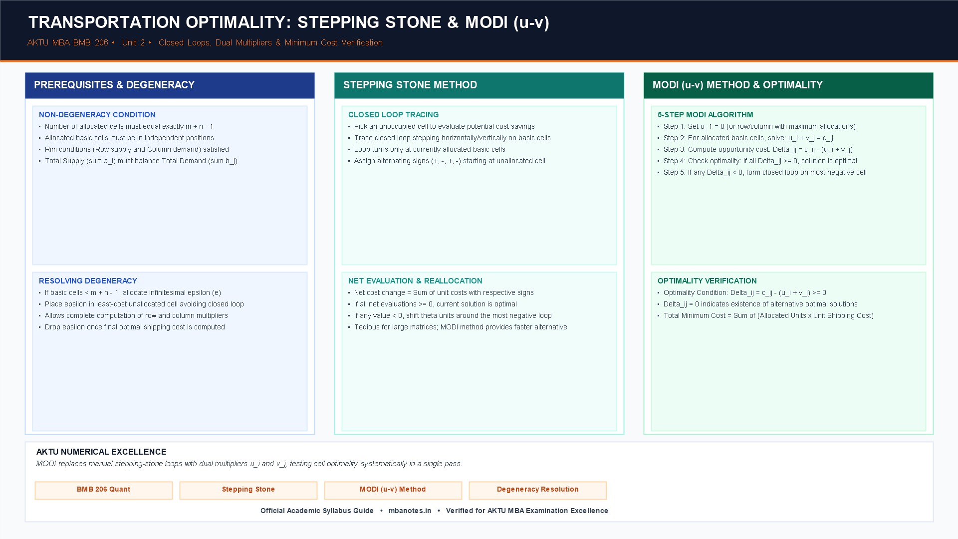
1. Optimality Testing in Transportation: Concept & Prerequisite Conditions
Once an Initial Basic Feasible Solution (IBFS) is generated (via VAM or Least Cost Method), operations research analysts must verify whether this solution is globally optimal. An initial solution may still leave substantial cost-saving opportunities unexploited.
Testing for optimality involves systematically answering one core question: ‘If one unit of product is shifted into an unoccupied cell, will the net total transportation cost decrease, remain unchanged, or increase?’
Prerequisite Conditions for Testing Optimality
- 1. Exact Basic Allocation Count ($m + n – 1$): In a transportation tableau with $m$ rows and $n$ columns, the number of allocated (occupied) cells must equal exactly $m + n – 1$.
- 2. Independent Positions (No Closed Loops): The occupied cells must occupy independent positions, meaning no closed horizontal-vertical loop can be formed solely among occupied cells. If a closed loop can be formed among occupied cells, the basic vectors are linearly dependent, violating linear programming feasibility.
- 3. Resolution of Degeneracy: If the number of occupied cells is strictly less than $m + n – 1$, the mathematical equations for dual variables ($u_i, v_j$) become algebraically unsolvable. Degeneracy must be resolved before proceeding.
Comparative Matrix: Stepping Stone Method vs. MODI (u-v) Method
| Operational Dimension | The Stepping Stone Method | The MODI (Modified Distribution) Method |
|---|---|---|
| Computational Nature | Geometric / visual tracing of closed paths | Algebraic formulation using dual potential variables ($u_i, v_j$) |
| Evaluation Workload | Must draw a distinct closed loop for EVERY single unoccupied cell | Solves dual equations once; computes $d_{ij} = c_{ij} – (u_i + v_j)$ directly |
| Loop Formation | Continuous loop drawing required across every iteration | Closed loop traced ONLY for the single incoming cell with most negative $d_{ij}$ |
| Efficiency on Large Matrices | Extremely tedious and error-prone for matrices larger than $3 \times 3$ | Highly scalable, mathematically elegant, and easily programmed in software |
| Optimality Condition | All loop evaluations are non-negative ($\Delta_{ij} \ge 0$) | All net evaluation indices are non-negative ($d_{ij} \ge 0$) |
| Managerial Utility | Pedagogical tool for understanding unit shifting mechanics | Universal standard utilized in commercial Operations Research solvers |
2. The Stepping Stone Method: Closed Loop Tracing & Reallocation
The Stepping Stone Method treats occupied cells as ‘stepping stones’ across a pond. The analyst evaluates the economic consequence of stepping into an unoccupied cell:
Rules for Tracing a Stepping Stone Closed Loop
- Select an empty cell to evaluate. This is the starting point of the loop.
- Trace a continuous path of alternating horizontal and vertical line segments connecting the starting cell back to itself.
- Every turning corner of the loop must turn strictly on an occupied (basic) cell. The path may jump over empty or occupied cells along a straight line, but changes in direction must occur at occupied cells.
- Assign alternating mathematical signs to the corners of the loop, starting with a plus sign ($+$) at the candidate empty cell: $(+, -, +, -)$.
- Compute the Net Evaluation Index ($\Delta_{ij}$): Add unit costs at cells with a plus sign and subtract unit costs at cells with a minus sign.
- If any $\Delta_{ij} < 0$, shipping along that path reduces total cost. Reallocate $\theta$ units around the loop, where $\theta$ equals the minimum allocation among cells marked with a minus sign ($-$).
3. The MODI (Modified Distribution / u-v) Method
The MODI Method (developed by George Dantzig) applies linear programming duality directly to the transportation tableau, bypassing the exhaustive manual task of tracing loops for every unoccupied cell:
The 5-Step MODI Computational Algorithm
- Step 1: Check Non-Degeneracy: Ensure total occupied cells equal $m + n – 1$.
- Step 2: Formulate Dual Equations for Occupied Cells: Assign dual variable $u_i$ to each row $i$ and $v_j$ to each column $j$. For every occupied cell $(i, j)$, set:
$$u_i + v_j = c_{ij}$$
This yields $m + n – 1$ equations in $m + n$ unknowns. Set the $u_i$ or $v_j$ associated with the row or column containing the most allocations to zero ($u_1 = 0$) and solve for all remaining $u_i$ and $v_j$. - Step 3: Compute Net Evaluation Index ($d_{ij}$) for Unoccupied Cells: For every empty cell $(i, j)$, calculate the opportunity cost:
$$d_{ij} = c_{ij} – (u_i + v_j)$$
- Step 4: Test for Optimality:
- If all $d_{ij} \ge 0$, the current transportation plan is Globally Optimal! Stop iterations.
- If any $d_{ij} = 0$, multiple (alternate) optimal solutions exist with the same minimum total cost.
- If at least one $d_{ij} < 0$, the solution is suboptimal and can be improved. Proceed to Step 5.
- Step 5: Reallocate Along Closed Loop: Identify the unoccupied cell with the most negative $d_{ij}$ (the incoming basic variable). Trace a single closed loop starting at this cell through occupied cells. Reallocate $\theta = \min(\text{allocations at } -\text{ corners})$, creating an improved transportation table. Repeat from Step 2.
MODI Optimality Equations & Solved Numerical Optimality Verification
Step-by-Step Solved Problem Illustration:
Problem Statement (AKTU Standard 10-Mark Optimality Numerical): Consider the Initial Basic Feasible Solution obtained via Vogel's Approximation Method for the cement distribution problem: Plants \(O_1, O_2, O_3\) and Warehouses \(D_1, D_2, D_3, D_4\). The 6 occupied cells and their allocations are: \((1, 2) = 300\) [cost \(c_{12}=1\)]; \((2, 1) = 250\) [cost \(c_{21}=2\)]; \((2, 3) = 150\) [cost \(c_{23}=5\)]; \((3, 2) = 50\) [cost \(c_{32}=3\)]; \((3, 3) = 250\) [cost \(c_{33}=3\)]; \((3, 4) = 200\) [cost \(c_{34}=2\)]. Test whether this initial plan is strictly optimal using the MODI (Modified Distribution) Method (\(u-v\) Method). If non-optimal, execute stepping stone path loop improvement; if optimal, state final distribution cost. Show resolution procedure if degeneracy occurs.
- Verify Non-Degeneracy Condition: Number of rows \(m = 3\); Number of columns \(n = 4\). Required allocations = \(m + n - 1 = 3 + 4 - 1 = 6\) cells. Number of occupied cells in VAM solution = 6. All 6 occupied cells are in independent positions (no closed loops). The solution is strictly non-degenerate! MODI method can proceed directly.
- Calculate Dual Potentials (\(u_i\) and \(v_j\)) for Occupied Cells: $\mathbf{u_i + v_j = c_{ij}}$
Let \(u_3 = 0\) (since Row 3 contains the maximum number of allocations: 3 cells).
• For Cell (3, 2): \(u_3 + v_2 = c_{32} \rightarrow 0 + v_2 = 3 \rightarrow v_2 = 3\);
• For Cell (3, 3): \(u_3 + v_3 = c_{33} \rightarrow 0 + v_3 = 3 \rightarrow v_3 = 3\);
• For Cell (3, 4): \(u_3 + v_4 = c_{34} \rightarrow 0 + v_4 = 2 \rightarrow v_4 = 2\);
• For Cell (1, 2): \(u_1 + v_2 = c_{12} \rightarrow u_1 + 3 = 1 \rightarrow u_1 = -2\);
• For Cell (2, 3): \(u_2 + v_3 = c_{23} \rightarrow u_2 + 3 = 5 \rightarrow u_2 = 2\);
• For Cell (2, 1): \(u_2 + v_1 = c_{21} \rightarrow 2 + v_1 = 2 \rightarrow v_1 = 0\).
Summary of Potentials: \(u = [-2, 2, 0]\); \(v = [0, 3, 3, 2]\). - Calculate Net Evaluation Index \(d_{ij} = c_{ij} - (u_i + v_j)\) for All 6 Unoccupied Cells:
• Cell (1, 1): \(d_{11} = 3 - [(-2) + 0] = 3 - (-2) = +5\);
• Cell (1, 3): \(d_{13} = 7 - [(-2) + 3] = 7 - 1 = +6\);
• Cell (1, 4): \(d_{14} = 4 - [(-2) + 2] = 4 - 0 = +4\);
• Cell (2, 2): \(d_{22} = 6 - [2 + 3] = 6 - 5 = +1\);
• Cell (2, 4): \(d_{24} = 9 - [2 + 2] = 9 - 4 = +5\);
• Cell (3, 1): \(d_{31} = 8 - [0 + 0] = 8 - 0 = +8\). - Audit Optimality Criterion: $\mathbf{d_{ij} = c_{ij} - (u_i + v_j) > 0 \quad \forall \text{ unoccupied cells}}$ Since every single net opportunity cost \(d_{ij}\) is strictly positive, no reallocation loop can reduce the transportation cost. The VAM basic solution is globally optimal and unique!
- State Final Optimal Schedule & Minimum Total Cost: $\mathbf{\begin{aligned} \text{Optimal Route: } & O_1 \rightarrow D_2: 300 \text{ bags} \times ₹1 = ₹300 \\ & O_2 \rightarrow D_1: 250 \text{ bags} \times ₹2 = ₹500 \\ & O_2 \rightarrow D_3: 150 \text{ bags} \times ₹5 = ₹750 \\ & O_3 \rightarrow D_2: 50 \text{ bags} \times ₹3 = ₹150 \\ & O_3 \rightarrow D_3: 250 \text{ bags} \times ₹3 = ₹750 \\ & O_3 \rightarrow D_4: 200 \text{ bags} \times ₹2 = ₹400 \\ \mathbf{\text{Minimum Total Cost}} &= \mathbf{₹2,850} \end{aligned}}$
- Method for Resolving Degeneracy: If an initial solution had only 5 allocations instead of 6 (\(m + n - 1 = 6\)), degeneracy would exist. Resolution Procedure: Select an unoccupied cell that has the minimum unit cost (\(c_{ij}\)) among empty cells AND does not form a closed loop with existing occupied cells. Allocate an infinitesimal quantity \(\varepsilon > 0\) (where \(\varepsilon\) is so small that it does not alter row supplies or column demands: \(250 + \varepsilon \approx 250\)). Treat this cell as an occupied cell, allowing all \(u_i\) and \(v_j\) potentials to be calculated. At final reporting, set \(\varepsilon = 0\).
4. Economic Significance of Transportation Dual Potentials ($u_i, v_j$)
The dual variables calculated in the MODI method possess direct managerial and financial significance:
- Location Advantage ($u_i$): Reflects the relative geographic advantage or disadvantage of plant location $i$. A lower $u_i$ indicates a strategically advantaged production site closer to major consumption hubs.
- Market Price Differential ($v_j$): Reflects the delivered value of the commodity at destination $j$. The difference $v_2 – v_1$ indicates how much more a buyer at Destination 2 should pay relative to Destination 1 to cover optimal distribution costs.
Non-Degenerate Basis
Verifying exact allocation count: Occupied Cells = m + n – 1 in independent non-loop positions.
Stepping Stone Loops
Tracing alternating (+, -, +, -) horizontal-vertical loops through occupied stones to evaluate empty cells.
The MODI (u-v) Method
Setting u_1 = 0, solving u_i + v_j = c_ij for basis cells, and auditing d_ij = c_ij – (u_i + v_j) ≥ 0 for optimality.
Degeneracy Resolution
Allocating infinitesimal quantity ε > 0 to the lowest cost independent empty cell to restore solvability.
6. Corporate Case Vignette: Corporate Case Vignette: Hindustan Unilever (HUL) Distribution Network Optimization
Background: Hindustan Unilever Limited (HUL), India’s largest FMCG corporation, operates a vast multi-tier manufacturing and distribution network supplying soaps, detergents, and personal care products from 28 manufacturing locations to over 40 central carrying-and-forwarding (C&F) depots across India.
The Logistics Optimization Challenge: Seasonal shifts in manufacturing capacity, diesel fuel price fluctuations, and highway freight contract renegotiations frequently made existing shipping routes suboptimal. HUL supply chain planners required an automated system to audit freight routing schedules for optimality every week.
The MODI Optimization Deployment: HUL’s logistics analytics group integrated the MODI Transportation Algorithm into its SAP Supply Chain Management platform:
- Generated initial feasible shipping plans using Vogel’s Approximation Method (VAM).
- Automated weekly MODI audits computing dual shadow prices ($u_i, v_j$) across all primary factory-to-depot transport links.
- When transport union strikes or highway disruptions increased costs on specific lanes, the MODI net evaluation index ($d_{ij}$) triggered automatic closed-loop freight reallocations.
Quantitative Results: The automated MODI optimization platform slashed primary freight spend by 4.2%, reduced cross-depot stock transshipments by 60%, and saved over ₹45 Crores in annual freight expenditures while maintaining a 99.4% on-time depot delivery service level.
7. AKTU Previous Years Questions & Model Solutions
The following questions reflect the official examination patterns, marks allocation, and rigorous mathematical evaluation guidelines of Dr. A.P.J. Abdul Kalam Technical University (AKTU) MBA Semester Examinations.
The optimality condition in the MODI method requires that the Net Evaluation Index (opportunity cost) for all unoccupied (non-basic) cells must be greater than or equal to zero: d_ij = c_ij – (u_i + v_j) ≥ 0 for all i, j. If all d_ij ≥ 0, the current transportation plan is globally optimal.
Degeneracy occurs when the number of allocated (occupied) cells in an m × n transportation tableau is strictly less than m + n – 1. It is resolved by allocating an infinitesimal positive quantity, epsilon (ε > 0), to one or more unoccupied cells with minimum cost that do not form a closed loop with existing occupied cells.
If d_ij = 0 for an unoccupied cell in an optimal transportation tableau, it indicates that an alternate (multiple) optimal solution exists. Shifting units into that cell will yield a different distribution schedule with the identical minimum total transportation cost.
Model Answer Structure:
1. Concept & Role of MODI: Introduce MODI as an algebraic application of linear programming duality that evaluates empty cells without drawing loops for each one.
2. Prerequisite Verification: Check non-degeneracy condition (Occupied cells = $m + n – 1$) and independence (no loops among occupied cells).
3. Dual Potentials Calculation: Set $u_1 = 0$ (or row with most allocations). Solve $u_i + v_j = c_{ij}$ for all basic cells.
4. Net Evaluation Matrix Computation: For each empty cell, calculate $d_{ij} = c_{ij} – (u_i + v_j)$. Present the complete matrix.
5. Optimality Audit: If all $d_{ij} \ge 0$, declare optimality. If any $d_{ij} < 0$, identify the cell with the most negative value as the incoming variable.
6. Loop Reallocation Mechanics: Draw the closed loop alternating $(+, -, +, -)$ at occupied corners. Determine $\theta = \min(- \text{ corners})$ and reallocate units.
7. Repeat & Final Solution: Show recalculation of potentials until all $d_{ij} \ge 0$. State the final optimal allocation and total cost.
Discussion & Questions
0 CommentsAcademic insights, questions, and conceptual clarifications from students & faculty.
No questions or comments yet
Have a doubt about this topic, an exam tip, or a conceptual perspective? Start the discussion below!
Leave a Comment / Ask a Question
Your email address will not be published. Required fields are marked *