
Sequencing Problem: Johnson’s Algorithm for n Jobs on 2 Machines, 3 Machines, and m Machines
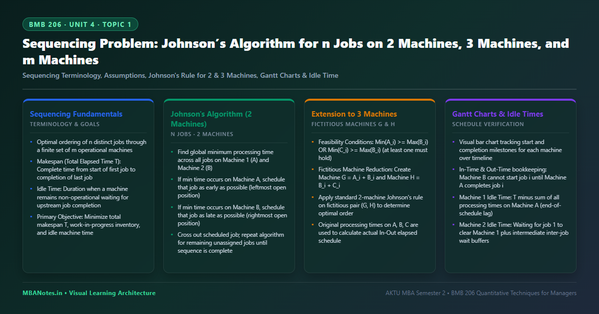
1. Conceptual Foundations & Terminology of Sequencing
Sequencing in operations management addresses the selection of an appropriate order in which a collection of jobs or work orders must be processed across a finite group of service facilities or machines. Without systematic sequencing, production lines experience excessive work-in-progress (WIP) inventories, unpredictable bottleneck delays, and severe machine under-utilization.
- Number of Machines ($m$): Refers to the distinct service stages or processing centers through which a job must pass in a specified technological route.
- Number of Jobs ($n$): Denotes the batch size of independent work orders awaiting service, where each job requires varying processing times on each machine.
- Processing Time ($t_{ij}$): The deterministic duration required by machine $j$ to completely execute and finalize job $i$.
- Total Elapsed Time ($T$ or Makespan): The complete chronological interval extending from the initiation of the first job on the first machine until the final exit of the last job from the terminal machine.
- Idle Time ($I_j$): The aggregate non-productive duration during which machine $j$ stands idle, waiting for upstream work pieces to complete processing or for setups to finalize.
- Flow Time of Job $i$: The total duration job $i$ spends inside the facility, comprising active machine processing time plus queuing and transfer wait times.
- No Passing Rule: The operational restriction dictating that all jobs must traverse machines in the exact same technological sequence without re-ordering between intermediate stages.
2. Core Assumptions and Operational Theorems
To guarantee mathematical tractability and permit algorithmic solutions via Johnson’s algorithm, the classical sequencing framework establishes several operational boundaries:
- Simultaneous Job Availability: All $n$ jobs are available for processing at time zero ($t = 0$), eliminating staggered arrival complications.
- Known and Deterministic Times: All machine processing times $t_{ij}$ are precisely known in advance and remain invariant regardless of sequencing choices.
- Single Machine Capacity: Each machine can process only one single job at any given instant; preemption or task splitting is strictly impermissible.
- Negligible Setup Times: Job setup times are either completely negligible or explicitly integrated into the reported processing times.
- Zero In-Process Transit Delay: The transfer time required to move a job from machine $j$ to machine $j+1$ is negligible or absorbed within operating intervals.
- Non-Preemptive Execution: Once a machine initiates processing on job $i$, it must run uninterrupted until the operation is fully completed.
- Inflexible Processing Path: Every job follows the identical technological progression ($M_1 \to M_2 \to \dots \to M_m$) without skipping any assigned station.
Mathematical Formulation & Solved Step-by-Step Numerical
Johnson’s Algorithm1. Johnson’s Rule for $n$ Jobs on 2 Machines ($M_1, M_2$)
Let $A_i$ and $B_i$ denote processing times of Job $i$ on Machine 1 and Machine 2 respectively.
Step 2a: If minimum is on Machine 1 ($A_k$), place Job $k$ in the FIRST available position.
Step 2b: If minimum is on Machine 2 ($B_k$), place Job $k$ in the LAST available position.
Step 2c: If tie occurs: break arbitrarily or favor smaller processing time on adjacent machine.
Step 3: Remove Job $k$ from matrix and repeat until all $n$ positions are filled.
2. Extension Rule for $n$ Jobs on 3 Machines ($A, B, C$)
A 3-machine problem can be converted into an equivalent 2-machine problem if at least one of these conditions holds:
Condition 2: $min_i (C_i) \ge max_i (B_i)$
If satisfied, construct fictitious machines:
$G_i = A_i + B_i \quad \text{and} \quad H_i = B_i + C_i$
Apply standard 2-machine Johnson’s rule on $(G, H)$ to obtain optimal sequence.
Five jobs $J_1, J_2, J_3, J_4, J_5$ must be processed through Machine 1 (Turning) and Machine 2 (Threading) in the order $M_1 \to M_2$. Determine the optimal sequence, construct the full In-Out schedule, and calculate total elapsed time $T$ and idle time for both machines.
| Job | $J_1$ | $J_2$ | $J_3$ | $J_4$ | $J_5$ |
|---|---|---|---|---|---|
| Machine 1 ($M_1$, hrs) | 3 | 12 | 5 | 2 | 9 |
| Machine 2 ($M_2$, hrs) | 8 | 6 | 4 | 9 | 3 |
Step-by-Step Algorithmic Execution:
- Iteration 1: The smallest processing time across the entire table is 2 hours for $J_4$ on Machine 1. Because it belongs to $M_1$, schedule $J_4$ in the first position:
[J4, _, _, _, _]. Eliminate $J_4$. - Iteration 2: The next smallest value is 3 hours, occurring twice: $J_1$ on $M_1$ and $J_5$ on $M_2$.
- For $J_1$ ($M_1$): Assign to the first available position $\to$ Position 2:
[J4, J1, _, _, _]. - For $J_5$ ($M_2$): Assign to the last available position $\to$ Position 5:
[J4, J1, _, _, J5].
- For $J_1$ ($M_1$): Assign to the first available position $\to$ Position 2:
- Iteration 3: The smallest remaining time is 4 hours for $J_3$ on $M_2$. Because it is on $M_2$, place $J_3$ in the last open slot $\to$ Position 4:
[J4, J1, _, J3, J5]. - Iteration 4: The remaining job $J_2$ automatically occupies Position 3:
[J4, J1, J2, J3, J5].
Optimal Processing Sequence: $J_4 \to J_1 \to J_2 \to J_3 \to J_5$
Makespan & Machine Idle Time Table:
| Scheduled Job | $M_1$ Time | $M_1$ In – Out | $M_2$ Time | $M_2$ In – Out | $M_2$ Idle Buffer |
|---|---|---|---|---|---|
| $J_4$ | 2 | 0 – 2 | 9 | 2 – 11 | 2 hrs (0 – 2) |
| $J_1$ | 3 | 2 – 5 | 8 | 11 – 19 | 0 hrs |
| $J_2$ | 12 | 5 – 17 | 6 | 19 – 25 | 0 hrs |
| $J_3$ | 5 | 17 – 22 | 4 | 25 – 29 | 0 hrs |
| $J_5$ | 9 | 22 – 31 | 3 | 31 – 34 | 2 hrs (29 – 31) |
• Total Elapsed Time (Makespan $T$): 34 hours
• Total Processing Time on $M_1$: $2 + 3 + 12 + 5 + 9 = 31\text{ hours}$
• Idle Time on Machine 1 ($I_1$): $T - \sum A_i = 34 - 31 = \mathbf{3\text{ hours}}$ (from hour 31 to 34)
• Total Processing Time on $M_2$: $9 + 8 + 6 + 4 + 3 = 30\text{ hours}$
• Idle Time on Machine 2 ($I_2$): $2\text{ hrs (initial wait)} + 2\text{ hrs (wait for } J_5) = \mathbf{4\text{ hours}}$
• Verification: Total $M_2$ runtime ($30\text{ hrs}$) + Idle ($4\text{ hrs}$) = $34\text{ hrs} = T$. (Exact Balance Confirmed!)
3. Comparative Analysis: Priority Dispatching vs. Johnson’s Algorithm
Industrial operations employ various heuristics when full algorithmic optimization is computationally impractical. Below is a rigorous comparison of Johnson’s algorithm against prevailing priority dispatching heuristics:
| Sequencing Technique | Governing Decision Rule | Primary Strength | Major Operational Limitation | Optimality Guarantee |
|---|---|---|---|---|
| Johnson’s Algorithm | Global minimum processing pairing; front-back allocation | Mathematically proven global minimum makespan ($T$) | Requires strict machine conditions for $m \ge 3$; deterministic data | 100% Proven Global Minimum |
| Shortest Processing Time (SPT) | Jobs sorted in ascending order of local processing duration | Minimizes mean job completion time and in-plant WIP inventory | Severely penalizes long jobs; causes inventory starvation downstream | Optimal for single machine mean flow |
| Earliest Due Date (EDD) | Jobs sequenced strictly by committed customer delivery deadline | Minimizes maximum job lateness and overdue penalty costs | Completely ignores machine idle times and total makespan duration | Suboptimal makespan |
| First-Come, First-Served (FCFS) | Sequential processing according to arrival order | Perceived customer fairness; trivial administrative overhead | Poorest performance in makespan, WIP accumulation, and machine idle times | Heuristic baseline only |
5. Corporate Case Vignette: Automotive Assembly Scheduling
Maruti Suzuki India Limited: Engine Block Machining Synchronization
At the Manesar powertrain manufacturing plant, Maruti Suzuki manufactures multi-cylinder engine blocks across two dedicated robotic machining centers: Station 1 (CNC Boring & Milling) and Station 2 (Honing & Precision Grinding). A batch of 6 customized engine block variants was scheduled on a traditional First-Come First-Served basis, yielding a daily makespan of 9.4 hours and generating 2.1 hours of idle time on the capital-intensive honing station.
The industrial engineering division implemented Johnson’s 2-machine algorithm. By front-loading engine blocks with minimal boring times and back-loading blocks with minimal honing cycles, the makespan contracted from 9.4 hours to 7.8 hours per batch. Idle time on the honing station fell by 68%, boosting line throughput by 180 engine units weekly without capital equipment investments.
6. AKTU University Examination Question Bank
Q1: Define Total Elapsed Time (Makespan) and Idle Time in machine sequencing.
Model Answer: Total Elapsed Time ($T$) is the total chronological time elapsed from the beginning of the first job on the first machine until the completion of the last job on the last machine. Idle Time ($I$) is the total unutilized duration for which a specific machine remains operational yet non-productive waiting for incoming workpieces.
Q2: State the necessary feasibility condition to reduce an $n$ jobs, 3 machines sequencing problem to an equivalent 2-machine problem.
Model Answer: The 3-machine problem ($A, B, C$) can be reduced to 2 fictitious machines ($G = A + B$, $H = B + C$) if and only if at least one of the following conditions is satisfied: (1) $min(A_i) \ge max(B_i)$, OR (2) $min(C_i) \ge max(B_i)$.
Q3: Explain Johnson’s algorithm for $n$ jobs on 2 machines. Solve the sequencing problem for jobs $J_1$ to $J_5$ with times on $M_1 = [5, 1, 9, 3, 10]$ and $M_2 = [2, 6, 7, 8, 4]$. Find optimal order, total elapsed time, and idle times.
Exam Strategy: Detail Johnson’s step-wise rule. Execute minimum search iterations. Construct the full In-Out scheduling table showing arrival and departure at each stage. Explicitly calculate $M_1$ and $M_2$ idle times and verify against total makespan $T$.
Discussion & Questions
0 CommentsAcademic insights, questions, and conceptual clarifications from students & faculty.
No questions or comments yet
Have a doubt about this topic, an exam tip, or a conceptual perspective? Start the discussion below!
Leave a Comment / Ask a Question
Your email address will not be published. Required fields are marked *