Queuing Theory: System Structure, Kendall’s Notation & Characteristics of (M/M/1) Model

⚡ 30-Second Revision SnapshotHigh Scoring • Quick Revision

Waiting Line Cause

Queues form because customer arrival rates fluctuate randomly even when long-term service capacity exceeds average demand.

Kendall’s Notation

Standard (A/B/c):(d/e) format. For (M/M/1):(infty/ FIFO), Poisson arrivals, Exponential service, single server, infinite capacity.

Formula & Metric

Key formulation: rho = (λ / mu) = (12 / 15) = 0.80 quad mathbf(80 % text Server Busy / Utilization). Master for exam numericals.

Traffic Intensity

rho = λ / mu. Steady-state stability requires rho < 1 (λ < mu); otherwise queue length expands indefinitely.

Little’s Laws

Fundamental bridge relations: Lₛ = λ Wₛ, L_q = λ W_q, and Wₛ = W_q + 1/ mu, establishing universal queue equilibrium.

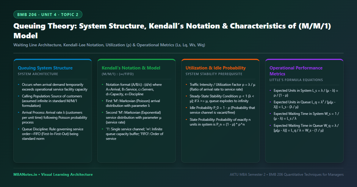
1. Queuing System Architecture & Structural Components

Queuing theory (waiting line theory) represents the mathematical investigation of delays and congestion experienced when customer demand temporarily outpaces operational service facility throughput. It provides managers with quantitative tools to strike a balance between customer waiting costs and facility capacity costs.

• Input Calling Population: The source population from which arrival entities originate. Classified as finite (e.g., breakdown of 10 factory machines) or infinite (e.g., retail shoppers entering a supermarket).
• Arrival Pattern ($\lambda$): The statistical frequency with which entities enter the system. Parameterized by arrival rate $\lambda$ (mean arrivals per unit time) or mean inter-arrival interval $1/\lambda$.
• Queue Discipline: The procedural prioritization rule governing which waiting entity is served next:
  • FIFO (First-In-First-Out): Standard equitable queuing order (e.g., ticket counters).
  • LIFO (Last-In-First-Out): Reverse order (e.g., cargo unloading from freight holds).
  • SIRO (Service In Random Order): Lottery or random pick.
  • Priority Service: Preemptive or non-preemptive urgent access (e.g., hospital trauma units).
• Service Mechanism ($\mu$): Comprises the number of parallel servers ($c$), arrangement of sequential phases, and average service rate $\mu$ (mean entities completed per unit time per server).
• System Capacity: The maximum allowable queue buffer limit. Infinite capacity permits unbounded lines, whereas finite capacity rejects arrivals once buffer saturation occurs (balking).
• Customer Behavioral Variations: Real-world waiting dynamics including Balking (refusing to join long queue), Reneging (leaving queue after waiting), and Jockeying (switching between parallel lines).

2. Kendall’s Notation & Model Assumptions

To universally classify waiting lines, British statistician D. G. Kendall formulated the shorthand notation $(A / B / c) : (d / e)$:

• $A$ (Arrival Probability Distribution): $M$ = Markovian/Poisson, $D$ = Deterministic, $E_k$ = Erlang-$k$, $G$ = General distribution.
• $B$ (Service Probability Distribution): $M$ = Markovian/Negative Exponential, $D$ = Deterministic, $G$ = General service distribution.
• $c$ (Number of Parallel Service Channels): $1, 2, \dots, \infty$.
• $d$ (System Capacity Limit): Maximum allowed customers in system ($\infty$ if unrestricted).
• $e$ (Queue Discipline): FIFO, LIFO, SIRO, or Priority.
• $(M/M/1) : (\infty / \text{FIFO})$ Foundational Assumptions:
  • Arrivals occur purely at random following a Poisson probability distribution with constant mean rate $\lambda$.
  • Service times follow an Exponential distribution with constant mean rate $\mu$.
  • A single server processes customers independently one at a time.
  • Waiting room capacity is infinite; no incoming customer is turned away.
  • The system is operating in steady-state equilibrium ($\lambda < \mu$, meaning $\rho < 1$).

3. Little’s Laws & System Performance Evaluation

Formulated by MIT professor John Little in 1961, Little’s Law provides a mathematically robust theorem applicable to almost any queuing system in steady-state, regardless of arrival distribution or service patterns:

• First Little’s Relation ($L_s = \lambda W_s$): The long-term average number of customers in a stationary queuing system equals the long-term average effective arrival rate multiplied by the average time spent inside the system.
• Second Little’s Relation ($L_q = \lambda W_q$): The long-term average number of customers waiting in the line equals arrival rate multiplied by the average queue waiting duration.
• Additive System Decomposition ($W_s = W_q + E(T)$): Total time in system cleanly decomposes into waiting time plus active service time ($1/\mu$).
• Sensitivity to Utilization ($\rho \to 1$): As traffic intensity approaches 1 ($100\%$), queue length does not grow linearly—it explodes exponentially toward infinity due to random clustering.

5. Corporate Case Vignette: Retail Bank Teller Optimization

6. AKTU University Examination Question Bank