Poisson and Exponential Distribution in Queuing Systems & Economic Optimization of Service Facilities

⚡ 30-Second Revision SnapshotHigh Scoring • Quick Revision

Poisson Arrival Process

Models discrete arrival counts in time t: P(k) = e^- λ t(λ t)^kk!, characterized by stationarity and independent increments.

Exponential Service ×

Continuous distribution density f(t) = mu e^- mu t modeling duration required to serve a customer, with mean time 1/ mu.

Formula & Metric

Key formulation: P(X = k) = e^- λ t(λ t)^kk! quad for k = 0, 1, 2, dots. Master for exam numericals.

Memoryless Property

P(T > s + t mid T > s) = P(T > t). Past waiting provides zero information regarding future service completion time.

Economic Cost Balance

Optimizes the trade-off curve between facility service capacity cost (Cₛ) and customer waiting penalty cost (C_w cdot Lₛ).

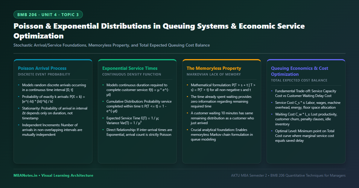
1. The Poisson Arrival Model: Axioms & Mathematical Properties

In real-world business and service systems, arrivals occur randomly rather than on rigid clockwork schedules. The Poisson process represents the quintessential stochastic model for counting discrete random events occurring over continuous time.

• Axiom of Stationarity (Homogeneity): The probability that an event occurs within a tiny time increment $\Delta t$ depends solely on interval length $\Delta t$ and mean rate $\lambda$, completely independent of the starting time $t$: $P(1\text{ arrival in }\Delta t) = \lambda \Delta t + o(\Delta t)$.
• Axiom of Non-Simultaneity (Orderliness): The probability of two or more simultaneous arrivals occurring within an infinitesimal interval $\Delta t$ is negligible: $P(\ge 2\text{ arrivals in }\Delta t) = o(\Delta t) \to 0$.
• Axiom of Independent Increments (Markovian Independence): The number of arrivals occurring in any two non-overlapping time intervals are statistically independent. Past arrival volume imparts zero predictive power on future arrival volume.
• Poisson Probability Mass Function: The probability that exactly $k$ entities arrive during a fixed observation window of duration $t$ is: $$P(X = k) = \frac{e^{-\lambda t}(\lambda t)^k}{k!} \quad \text{for } k = 0, 1, 2, \dots$$
• Equivalence of Mean and Variance: For any Poisson arrival distribution, the expected value and the variance are strictly identical: $E(X) = \text{Var}(X) = \lambda t$.

2. Negative Exponential Service Times & The Memoryless Theorem

While arrivals represent discrete event counts, service duration is a continuous random variable $T$. When arrivals follow a Poisson distribution with parameter $\lambda$, the elapsed time between consecutive arrivals (inter-arrival time) is mathematically proven to follow a Negative Exponential distribution with parameter $\lambda$. Similarly, service duration across varied transactions is modeled via the Exponential distribution:

• Probability Density Function (PDF): $f(t) = \mu e^{-\mu t}$ for $t \ge 0$, where $\mu$ denotes the mean service completion rate per unit time.
• Cumulative Distribution Function (CDF): The probability that a service operation completes within time $t$ is: $$P(T \le t) = int_0^t \mu e^{-\mu x} dx = 1 - e^{-\mu t}$$
• Tail Survival Function: The probability that service requires more than time $t$ is $P(T > t) = e^{-\mu t}$.
• Expected Value & Variance: Mean service time is $E(T) = (1 / \mu)$, and variance is $\text{Var}(T) = (1 / \mu^2)$.
• The Memoryless (Markovian) Property: The Negative Exponential distribution is the only continuous probability distribution that possesses complete lack of memory. Formally: $$P(T > s + t \mid T > s) = (P(T > s + t) / P(T > s)) = \frac{e^{-\mu(s + t)}}{e^{-\mu s}} = e^{-\mu t} = P(T > t)$$ Managerial Implication: The fact that a transaction has already been in progress for $s$ minutes gives zero predictive information regarding how much further time will be required to finish. The remaining duration has the exact same probability distribution as a brand new transaction.

3. Economic Analysis of Queuing Systems: The Cost Trade-off Model

From an executive management standpoint, queuing models exist to resolve an economic conflict between two opposing cost curves:

• Cost of Providing Service Capacity ($C_s cdot s$): The direct capital, operational, and labor expenditures required to install and maintain service channels (e.g., teller salaries, automated machinery, maintenance, server hardware). This cost increases linearly with the number of servers or service speed $\mu$.
• Cost of Customer Waiting ($C_w cdot L_s$): The tangible and intangible losses incurred due to delay (e.g., driver idle wages, in-transit inventory holding costs, customer frustration, brand abandonment, penalty clauses). This cost is a convex decreasing function of capacity.
• Total Expected System Cost Function ($\text{TEC}$): $$\text{TEC}(s) = \text{Total Service Cost} + \text{Total Waiting Cost} = (C_s \times s) + (C_w \times L_s)$$
• Optimal Economic Service Capacity ($s^*$): The service capacity or number of channels that minimizes Total Expected Cost ($\text{TEC}$), occurring precisely at the inflection point where marginal service investment equals marginal reduction in waiting penalties.

4. Comparative Analysis: Deterministic vs. Stochastic Queues

Understanding why queues build up even when capacity exceeds demand requires contrasting deterministic models with stochastic waiting realities:

6. Corporate Case Vignette: Logistics Hub Container Cranes

7. AKTU University Examination Question Bank